
Mind Over Markets CHAPTER 3 - Advanced Beginner
When David reached the advanced beginner stage, he could play a few simple songs all the way through. Then his instructor gave him a new song to learn that was in a different key signature, explaining that certain notes are raised and must be played on the black keys. When David tried to play it, he became frustrated and exclaimed, “This song doesn’t work.”
He was playing every note as it was written, the way he had learned as a novice. The instructor calmly explained that in any key signature besides C major, certain notes must be played differently.
David fell victim to tunnel vision, for he was thinking only of the limited rules he had memorised and was not incorporating the new information in his playing. He then blamed the written music to explain his failure and frustration. The musical score is not right or wrong; it is only a passive medium that communicates a certain piece of music. Tunnel vision is an easy trap to fall into, especially when learning large amounts of new information. It is not uncommon to hear beginning Market Profile traders comment, “The Profile doesn’t work.” There is nothing about the Profile that does or does not work. It is only a passive gauge of market-generated information—a way to organise the data, much like the musical score. What fails to work is the trader’s ability to see the big picture objectively and realise that everything is a series of facts surrounded by other circumstances. Only when all the circumstances are interpreted together and a holistic image develops will successful trading occur.
Building the Framework
In Advanced Beginner, we will begin to build upon the foundation established in Novice. You will learn many of the broad concepts that will serve as tools for building a framework for understanding the marketplace through the Market Profile.
The Big Picture: Market Structure, Trading Logic, and Time
The big picture is made up of three broad categories of information: market structure, trading logic, and time. As a novice you learned the basics of market structure, the most tangible information offered by the Market Profile in the unique bell curve graphic. Very short-term structure is reflected through time price opportunities (TPOs) and the market’s half hour auctions. As the day progresses, the market begins to form one of the day types through range extension, tails, etc.
We can see, measure, and name the physical aspects of the Profile. By the day’s end, structure shows not only what happened, but also when it happened and who was involved. In short, market structure provides visible evidence of the actions and behaviour of the market’s participants.
In this section, this structural evidence will be built upon and combined with time and trading logic. Time is the market’s regulator. In its broadest sense, time sets limitations on the day’s trading by imposing a certain framework (i.e., the number of hours from the open to the close). Most traders see time only in its function of the closing bell, and do not consider its influence on price and opportunity. Without considering time, there is no way to judge value, and trading becomes a 50/50 gamble on price movement.
In the day timeframe, time validates price. The areas of the Market Profile’s bell curve showing the greatest depth indicate the prices where trading spent the most time, thus establishing value for that day (price * time = value).
Understanding value and value areas will become more and more important as we progress through the learning process.
Time also regulates opportunity. Consider an everyday life example. You are in the market to buy a pair of snow skis. You shop around long enough to get a good feel as to how much skis normally cost or what you consider value. You don’t need the skis right away, so you wait for a chance to buy them under value—you are a long-term buyer.
You know that after the ski season ends, most stores will have summer ski clearance sales, when price will temporarily drop below value. You also know that these prices will not last long, for time regulates opportunity. The stores could not afford to sell at such low prices all year and still make a profit. They are merely clearing excess inventory in preparation for new stock. To take advantage of the low price, you must act quickly.
The same principle is true in the futures market. Good opportunities to buy below value or sell above value will not last long, for price will move quickly with increased competition. If price stays below value for a long time, for example, it is no longer a good opportunity. Something has changed, and value is being accepted lower.
The third and most difficult category is trading logic. Trading logic is largely a product of experience, but it is more than just careful observation and practice; it is an understanding of why the market behaves the way it does. This understanding is best gained over time and through a conscious effort to understand the forces behind market movement. Certain aspects of trading logic can be taught in relation to structure and time, by derivative learning. For example, you know that a tail is an indicator of strong other timeframe activity on the extremes. If the tail is “taken out” by a price rotation back into the tail and TPOs build over time, trading logic says that something has changed, and the other timeframe buyer or seller that moved price quickly is no longer present or is less willing to respond to the same price levels.
The only way to really understand the market and its logic is to observe, interpret, and trade. Remember, much learning does not teach understanding. We will be integrating trading logic throughout the remainder of the book.
A Synthesis: Structure, Time, and Logic
Imagine two children, each racing to complete a giant jigsaw puzzle. Both are working on the same puzzle with an equal number of pieces (the same structure), but one child has a picture of the finished puzzle and one does not. Obviously, the child with knowledge of the whole picture will finish first.
The Profile graphic is much like an intricate puzzle. Its structure reveals more and more as the day nears completion. But, like the child with a picture of the finished puzzle, traders with an understanding of the big picture—those that can see the market develop before it is revealed by structure—are generally the first to put together the pieces of the market. Market time and trading logic are the two big-picture components of a whole-market understanding. Only through a synthesis of all three components will a trader successfully put together the puzzle. We will now discuss market structure, time, and trading logic according to five general criteria:
1. Ease of learning
2. Amount of information
3. Recognition speed
4. Trade location
5. Confidence level
Ease of Learning Ironically, the order in which structure, time, and logic are usually learned is opposite from their order of occurrence in the marketplace—not because they are taught incorrectly, but rather because market structure is learned more quickly and easily than the roles of time and logic. Market structure is the finished product, and it is always easier to see the finished product than to identify the stages of its assembly. Mastering market structure is largely a matter of successfully recognizing and interpreting the Profile graphic. Understanding the role of time, however, requires a much deeper understanding of the market’s auction process. Trading logic is the hardest to learn, particularly from a book or instructor, for logic is the ultimate outcome of trading practice and experience. Trading logic is the raw human instinct of the marketplace. True trading logic comes only through intensive participation and careful examination of real market situations.
Amount of Information While market structure is clearly the most tangible information offered by the Profile, it also contains the greatest amount and variety of information. Why, then, is it so difficult to interpret market structure in real trading situations? It is relatively simple to recognize and interpret the day’s final structure. The difficulty lies in recognizing what is transpiring as the structures are building.
The inability to identify a developing structure does not necessarily mean that the information is lacking. It is simply not conveyed in an easily readable format. In addition, it is possible to monitor the wrong information. Market time and trading logic provide very little in terms of visible, tangible information—but the information is in the market. Successful trading requires the ability to find and interpret the more subtle clues found in time and logic, and integrate them with the developing structure.
Recognition Speed It takes time to build structure. Thus, while the Profile structure reveals a lot, the sheer fact that time must transpire suggests that fundamental changes occur in the market before they are revealed by structure. Structure acts as the market’s translator, and translated information is second-hand information. The market has already spoken in the form of time and logic. Traders who rely exclusively on structure without integrating time and logic will be late in entering and exiting the market, just as a catcher who holds his throw until he sees how fast a man stealing second base can run will never make the out.
Trade Location Later recognition leads to later entry and exit, which in turn leads to less desirable trade location. For example, range extension (structure) confirms that other timeframe buyers have entered the market. But when did they enter the market? If We rely solely on structure, we do not realise the other timeframe buyer’s point of entry until the point of range extension—that is, when price is on the day’s high. Buying the high results in poor day timeframe trade location, at least temporarily. In many cases, it is possible to know that buyers are assuming control before the actual structural confirmation (range extension) through an understanding of market time and trading logic.
Confidence Level Trading based on structure provides the greatest level of comfort and confidence, for there is obvious proof on which to base a decision. The more information we have in our favour, the more comfortable we are with a trade. Unfortunately, visible information and opportunity are inversely related. The more structural information present, the less an opportunity still exists. Thus, if a trader waits for too much information, chances are good that the real opportunity has been missed. If all the evidence is present and visible, then you are far from the first to have acted on it and probably have poor trade location.
Market time, followed by trading logic, provides the least amount of visible evidence. To the advanced beginner trader, trades based on time and logic offer a lower level of confidence, for the trader is not yet comfortable outside the realm of structure. Seasoned traders with a whole-market understanding, on the other hand, trade using logic and time and then monitor activity for the additional information (structure) necessary to increase their confidence in the trade.
Summary Logic creates the impetus, time generates the signal, and structure provides the confirmation.
The preceding discussion delineates the many differences among structure, time, and logic, but the answer to a practical sense of their synthesis must be developed through time and experience. Such coordination is gained only through observing and acting on market-generated information every day (doing the trade). Although the Market Profile is best known for the Profile graphic, or structure, experience has shown that understanding the influence of time and trading logic is more important to reaching a holistic view of the marketplace. Putting in the extra effort to fully understand the building blocks of structure—market time and trading logic—will better prepare traders to anticipate and take advantage of trading opportunities as they develop, not after they have passed.
Evaluating Other Timeframe Control
We have stressed in general terms the importance of determining who, if anyone, is in control of the market. Let us now enter into evaluating other timeframe control in a more detailed, conclusive discussion. The elements that signify other timeframe control are perhaps the most deceptive of all market-generated information we will cover. Often, information that we believe we are interpreting objectively is presented in such a way that its actual nature is misinterpreted.
An example of such an illusion often occurs when a market opens exceptionally above the previous day’s value area.
The other timeframe seller responds to the higher open, enters the market aggressively, and auctions price lower all day.
However, at the conclusion of the trading session, the day’s value is ultimately higher. In the day timeframe,
other timeframe sellers dominated the market’s auctions through their attempts to return price to previously
accepted value. But the responsive selling was not strong enough to completely overpower the higher
opening triggered by a strong other timeframe buyer. Day timeframe structure indicated weakness,
while the market was actually very strong in the longer term.
As illusions go, the preceding example is relatively easy to detect and evaluate.
Unfortunately, the information generated by the market is not always so clear.
In most cases, a more analytical approach is needed to effectively gauge who is winning the battle
for control between the other timeframe buyer and seller.
To evaluate other timeframe control, we will examine range extension, tails, activity
occurring in the“body” of the Profile, and value area placement in relationship to the previous day.
In addition, each of these factors will be studied further, based on whether the participants are
acting on their own initiative or are willing to act only in response to an advantageous market movement.
Another timeframe participant who acts on his own initiative is usually more determined than one
who merely responds to a beneficial opportunity.
This section will deal with evaluating who has control in the day timeframe.
The ability to process information through the Profile structures enables a
trader to recognize attractive day timeframe trades. Long-term traders must also be able to read and interpret
day timeframe structure, for a long-term auction is simply a series of day auctions moving through time.
Long-term auction evaluation and value area placement requires far more analysis and will be detailed in
Chapter 4. We mention it here to avoid creating the illusion that day timeframe
control is all conclusive—it merely reflects activity occurring during one day in the life of a longer-term auction.
Learning to read and interpret day timeframe structure is beneficial to all market participants at one time
or another. This understanding most obviously influences the individual who trades only in the day timeframe
—in other words, one who begins and ends each day with no position. However, all long-term traders are
also day traders on the day that they initiate or exit a trade. The concept of longer timeframe participation
in the day timeframe is best expressed through two examples.
Imagine a food company that purchases a large amount of corn for its cereal processing plant.
The food processor has an opinion that corn prices will rise but also wants to be appropriately
hedged against loss. Thus, as the price of corn rises, the company gradually sells grain futures
against its inventory, in effect scaling in a hedge. On one particular morning, corn opens far
above the previous day’s value, but early Profile structure indicates weakness. The processor
takes advantage of the higher open and expands the size of its hedge (by selling more futures).
However, as price auctions lower over the course of the day, the processor may partially close
out its shorts, seeking to replace them later at higher prices. The food company’s hedging goals
are clearly long term. However, when the market created an opportunity in the day timeframe,
the food company elected to trade a portion of the hedge.
In a second example, a futures fund manager with a bullish bias may elect to trade around his long-term
positions by taking advantage of day timeframe structure. If market structure indicates that the market
is likely to break, he may sell a percentage of his position, reestablishing it later in the day. In fact, if
there is enough volatility in the market, he may reposition a portion of his inventory more than once
on the same day. Putting aside the longer term for a later section, we will now begin the discussion
of other timeframe control in the day timeframe.
Other Timeframe Control on the Extremes
Tails (or Extremes)
Tails are created when an aggressive buyer or seller enters the market on an extreme and quickly moves price.
Generally, the longer the tail, the greater the conviction behind the move (a tail must be at least two TPOs
long to be significant). A tail at the upper extreme of a day’s profile, for example, indicates a strong other
timeframe seller entered the market and drove price to lower levels. In terms of other timeframe control,
no tail may also be significant. The absence of aggressive other timeframe activity on an extreme indicates
a lack of buyer or seller conviction.
Range Extension
Range extension is another structural feature that identifies control and helps gauge buyer/seller strength.
Multiple period range extension is generally the result of successively higher or lower auctions.
The stronger the control, the more frequent and elongated the range extension, resulting in a more
elongated Profile (an elongated Profile is an indication of good trade facilitation). In a Trend day,
for example, the other timeframe’s dominance is clearly evident through continued range extension
and price movement throughout the day.
Other Timeframe Control in the Body of the Profile
The role of the larger institutions and commercial participants in the marketplace is much greater than
merely seeking to take advantage of price as it moves away from value (evidenced by tails and range extension).
Many of the long-term commercial users of the futures exchange have a certain amount of business they
must conduct every day. For example, General Mills must put boxes of cereal on millions of breakfast
tables every morning. Therefore, they are constantly in the market as part of their daily business.
This more subtle, involuntary other timeframe activity generally takes place within the body of the Profile.
Nonetheless, it plays an important part in our evaluation of the competition that goes on between the other
time frame participants. The TPO count provides a means of measuring the activity of the other timeframe
within the body of the day’s Profile.
TPO
Count the Time Price Opportunity as the smallest unit of market measurement. As mentioned earlier,
TPO stands for Time, the market’s regulator, and Price, the market’s advertiser, together creating the
Opportunity to buy or sell at a given price at a particular time. Monitoring the TPO count helps evaluate
other timeframe control within the developing value area. Specifically, the TPO count measures the level
of imbalance (when such an imbalance exists) between the other timeframe participant and the day
timeframe (mostly local) trader.
The key to understanding how an imbalance can occur is to recognize that the other timeframe buyer does not
deal directly with the other timeframe seller. Recall that the local, or scalper, acts as a middleman between
these two long-term participants. Thus, the other timeframe buyer generally buys from a local, and the other
timeframe seller typically sells to a local.
Imbalance occurs when there are more other timeframe buyers than sellers or more other timeframe sellers
than buyers, leaving the local with an imbalance. Before we can learn how to measure this imbalance,
we must first gain a better understanding of how the locals conduct their business.
The locals position themselves between the flow of outside buy orders and outside sell orders
(orders placed predominantly by off-floor, other timeframe participants). For example, suppose
that a floor broker receives an order to sell 100 contracts at, say, $5.00 per contract. The locals
would buy the contracts from the broker and then turn around and sell them to another floor broker
who has an order to buy 100 contracts at $5.02. In this situation, the locals perform their role of
facilitating trade and, in return, receive a small margin of profit.
The trade facilitation process is seldom so ideal, however. Often there are more other timeframe buyers
than sellers—causing the local’s inventory to become overloaded. For example, if an usually large number
of sell orders enter the pit, the local’s inventory begins to accumulate to a point where he gets “too long.”
In other words, the local has purchased too much from the other timeframe seller.
If the other timeframe buyer does not appear relatively quickly, the local must bring his inventory back into
balance in some other way. One’s first thought would be that the local simply needs to sell off his excess
inventory. However, this is not so easy, for reversing and selling would only serve to accentuate the selling
that is already flowing into the market. Therefore, his first priority is to stop the flow of outside sell orders
by dropping his bid in hopes that the market will stabilise and he can balance his inventory. If lower prices
do not cut off selling, the local may then be forced to “jump on the bandwagon” and sell (liquidate) his
longs at a lower price.
Viewed from another perspective, suppose you decided to try to make extra spending money by scalping
football tickets. A month before the chosen game, you purchased 20 tickets from the box office at $10
each. In this case, the box office is the other timeframe seller and you are the day timeframe buyer.
Over the ensuing month, your team loses every game and slips from first to fifth place. Not surprisingly,
the attendance is dismal on the day of the game at which you intend to sell your tickets.
Few other timeframe buyers (fans) show up. In order to get rid of your inventory and recover
at least part of your costs, you are forced to sell your tickets at $8 instead of $12 or $15. In this
example, there were more other timeframe sellers than buyers. Consequently, prices had to move
lower to restore balance.
The same concepts apply to the futures marketplace. If we can identify imbalance before it corrects
itself, then perhaps we can capitalise on it, too. Tails and range extension are more obvious forms
of other timeframe presence, but on a volatile or choppy day, much of the imbalance occurs in more
subtle ways within the value area. The TPO count is an excellent method for evaluating day-to-day
imbalance that occurs within the developing value area.
The TPO count is found by isolating the point of control (the longest line closest to the centre of the range),
summing all the TPOs above it and comparing that number to the total number of TPOs below it.
Single-print tails are excluded from the count, because their implications are clear and have
already been considered when examining activity on the extremes. Remember, the point
of control is significant, because it indicates the price where the most activity occurred
during the day and is, therefore, the fairest price in the day timeframe (price * time = value).
Figure 3.1 illustrates the TPO count.
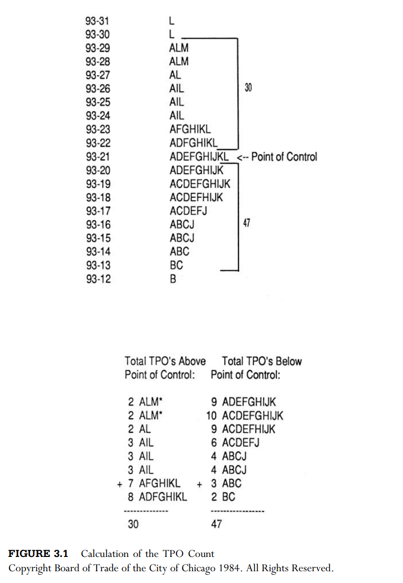
The total TPO figure above the point of control represents other timeframe traders willing to sell and stay short above value, while total TPOs below the point of control represent other timeframe traders willing to buy and stay long below value. The resulting ratio is an estimate for buyer/seller imbalance in the value area. For example, a ratio of 32/24 breaks down to 32 selling TPOs above the point of control, and 24 buying TPOs below. Note that a value area is not specifically calculated. Rather, the methodology of the TPO count (i.e., single-print rejections are not counted) implies value.
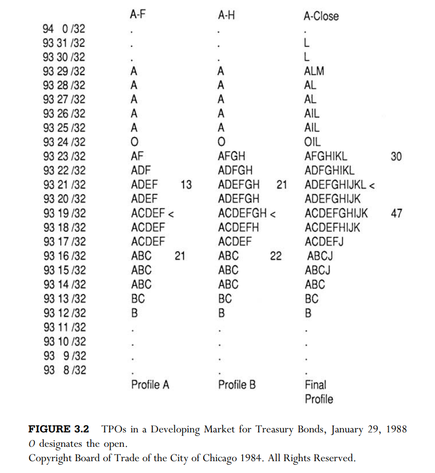
Portrayed in Figure 3.2 are three developing versions of the Treasury bond Profile of January 29, 1988. Profile A displays time periods A–F of the day. The 29th saw an opening substantially higher than the close of the previous day, followed by an early-morning sell-off as price attempted to auction down.
As the trading day proceeds, however, our concern is with discovering exactly who is more aggressive
(who is in control) within the developing value area. Occasionally, activity reflected by range extension
and tails will give us some clues regarding which participant is more aggressive on the extremes
. But the value area battles are more subtle and often much slower to develop. Monitoring the
TPO count through time helps us measure how the wins and losses are stacking up and gives
some indication of who will be the victor in the battle for control in the body of the Profile.
Examine Profile A again. A to F period registers a 13/21 TPO count, which favours the other timeframe buyers. Consider what this 13/21 TPO count logically means: The fact that the TPO count below the point of control is growing larger indicates that, although price is spending time below the point of control, price is not going anywhere.
Had other timeframe sellers been aggressive within the value area, there would have been downside range extension. Range extension would have lowered the point of control (and the perception of value), therefore balancing the TPO count and quite probably shifting it in favour of the sellers. With a TPO count building in the bottom half of the value area (buyers) and no selling range extension, chances are that it is the floor traders, or locals, who are selling to the other timeframe buyers.
Profile B in Figure 3.2 shows the TPO count through the H period moving back into balance at 21/22. This temporary return to balance indicates that the locals’ inventories became too short—in essence, they had sold too much—and were forced to cover (buy back) some of their shorts to bring their inventories back into line. Consequently, prices rotated up in G and H periods, as the locals restored balance to their inventories.
Again, in the final Profile, other timeframe sellers were not present as price continued to rotate toward the day’s upper extreme. The L period TPO print at 93 21/32 (bonds trade in 32nds of $1,000), and subsequent L period range extension pulled the point of control higher, confirming a final TPO tally in favour of buyers, 30/47. This end-of-the-day imbalance often provides momentum into the following day.
Initiative versus Responsive Activity
Knowing whether the other timeframe participants are acting on their own initiative, as opposed to responding to opportune prices is also important to understanding their influence. Traders can determine if activity is initiative or responsive by comparing the relationship of the day’s structure to the previous day’s value area. The previous day’s value area acts as the truest, most recent indication of a level where price has been accepted over time. Four types of potential activity may emerge:
1. Initiative buying
2. Initiative selling
3. Responsive buying
4. Responsive selling
Briefly, initiative buying is any buying activity occurring within or above the previous day’s value area. Conversely, initiative selling is any selling activity that takes place within or below the previous day’s value area. Initiative activity indicates strong conviction on the part of the other timeframe.
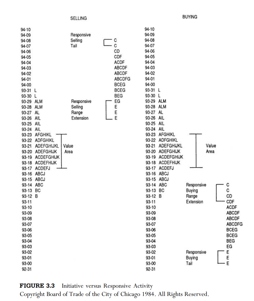
Responsive activity is the opposite of initiative activity. Buyers respond to price below value, and sellers
respond to price above value. Figures 3.3 and 3.4 illustrate these concepts in detail. Looking first at the
lower right-hand side of Figure 3.3, the upward range extension in C period and the E period buying
tail represent responsive buying. Buyers are responding to price considerably below the area of recent
price acceptance. In other words, buyers have responded to the opportunity to buy cheap. Keep in mind
that if price auctions down and finds buyers, that alone is not responsive. It is the fact that price is below
value that makes the buying responsive.
A responsive buying tail is also initiative selling range extension. For example, when the grocer lowered prices in his peanut butter extravaganza, it created initiative selling range extension. Buyers responded to this price below value, returning price to previous levels in a responsive buying tail. The initiative range extension and the responsive tail were one and the same activity.
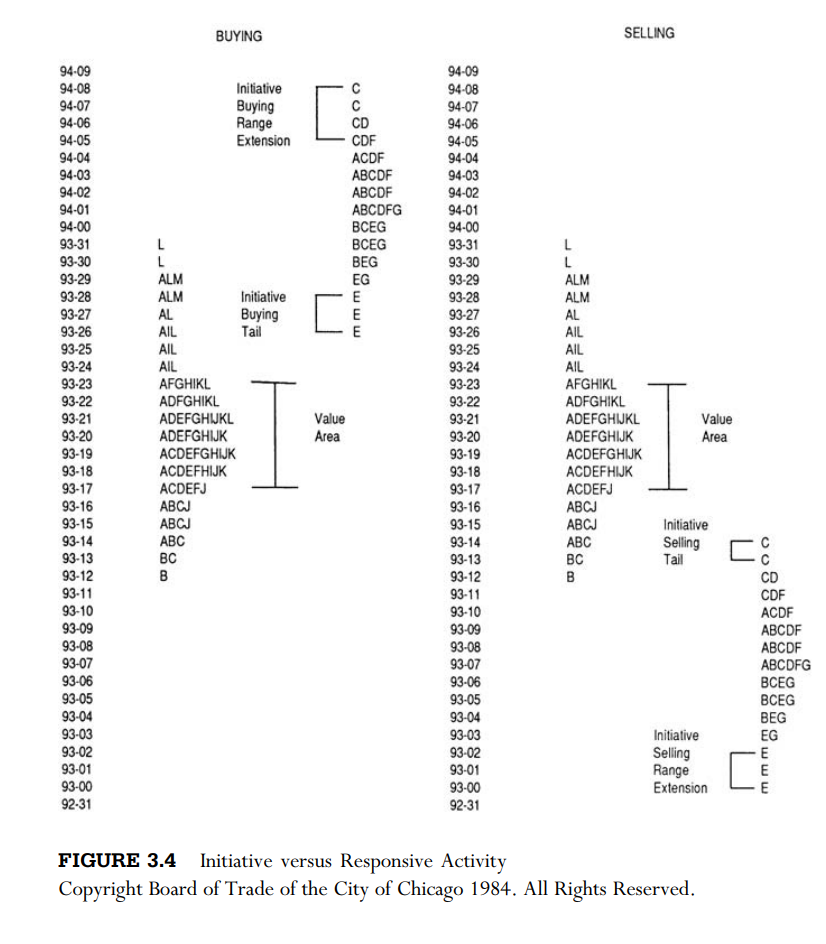
Referring again to Figure 3.3, notice that the flipside of the C period responsive buying range extension is a C period initiative selling tail. Similarly, the E period responsive buying tail was actually the outcome of a harsh rejection of E period initiative selling range extension. In Figure 3.4 we find the same thing: C period initiative buying range extension meets a responsive seller and eventually becomes a responsive selling tail. If range extension occurs in the last period of the day, however, it does not indicate a tail as well. A tail is only valid when confirmed by a rejection of price in at least one additional time period.
Range extension and tails occurring within the previous day’s value area are also considered initiative. If people choose to buy or sell within the area of
most recently perceived value, their free choice to agree with recent price levels is really an initiative decision in itself, for they are not responding to excess price. Like all the information you are learning, the concept of initiative and responsive action is not just a random designation that should be committed to memory, but rather a logical characterization of price’s relationship to value.
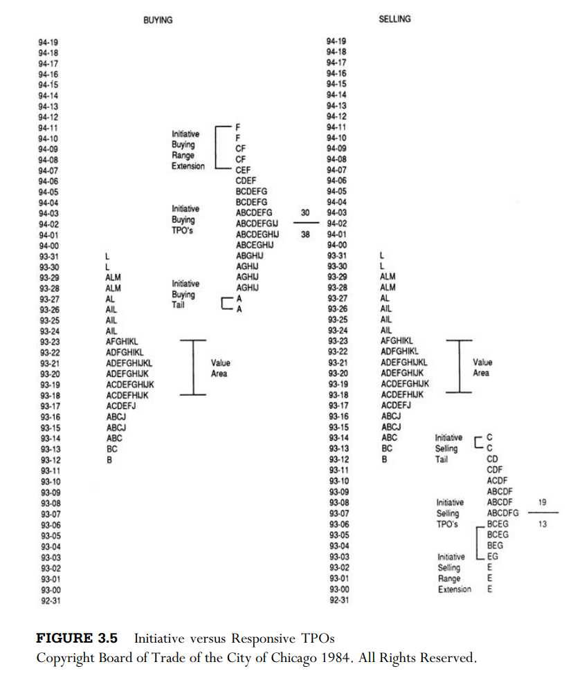
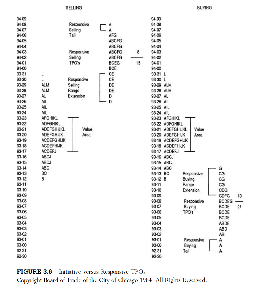
The entire day’s value area can be classified as either initiative or responsive as well. As noted before,
this identification is important because it gives the trader an indication of market conviction and confidence.
In short, initiative buying and responsive selling TPOs occur above the previous day’s value area,
while responsive buying and initiative selling TPOs occur below the previous day’s value area.
Any TPO activity occurring within the previous day’s value area is considered initiative,
although it does not carry as much confidence as initiative activity that takes place outside of the
value area. Figures 3.5 and 3.6 illustrate these concepts.
Trending versus Bracketed Markets
Understanding the dynamics of trending and bracketed markets, and the transition from one to the other, is one of the most difficult auction market concepts to grasp. In a very real sense, this could be due to the fact that such an understanding requires a firm grasp of overall market behaviour, as well as the synthesis of a large part of all Profile knowledge. For this reason, we lay the groundwork of trending and bracketed markets here, with a more detailed discussion to follow in the Competent section.
Let us begin with a few common dictionary definitions of a trend and a bracket in order to form a basic mental image of the two. Webster’s New Collegiate Dictionary defines a trend: (a) “to extend in a general direction: follow a general course . . . to show a tendency,” or (b) “the general movement in the course of time of a statistically detectable change; also: a statistical curve reflecting such a change.” Unfortunately, there is no absolute way to define a trend, for it is a function of the market and your trading timeframe.
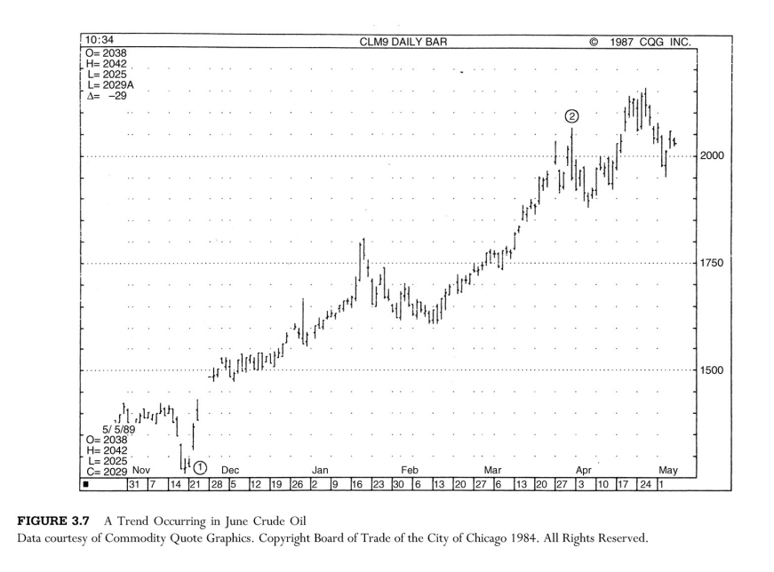
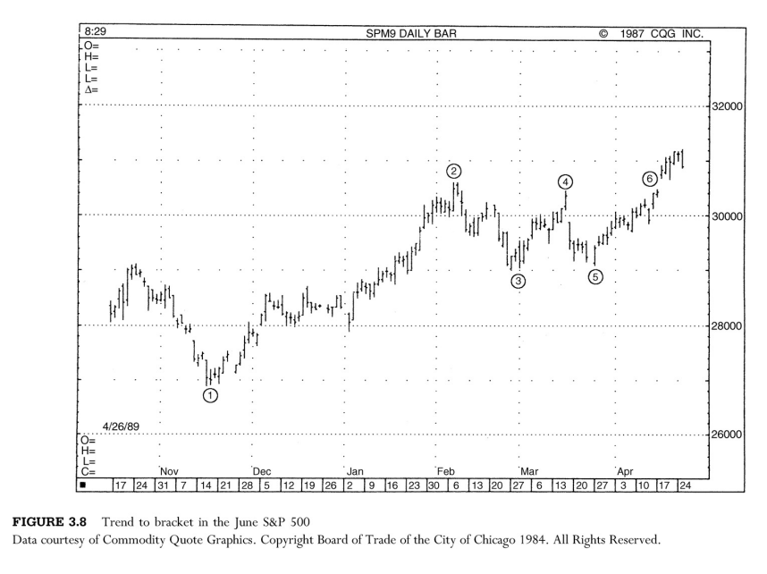
A trend, put simply, is a divergence of price away from value. For our purposes, the price divergence in a trend is characterised by a series of day auctions (value areas) moving in a clear direction over a long period of time. An example of such a long-term trend is illustrated between points 1 and 2 in the daily bar chart for Crude Oil in Figure 3.7. Figure 3.8 displays another trend occurring in the S&P 500 (between points 1 and 2) that ends in a bracket.
Webster defines bracket: (a) “to place within or as if within brackets,” or (b) “to establish a margin on either
side of.” A bracketed market is a series of price movements contained “as if within brackets.”
The market auctions back and forth between two price levels that serve as a margin on either
end of the range. Referring to Figure 3.8 again, the S&P market began the bracketing process at point 2,
then auctioned back and forth within the bracket enclosed by points 2 through 6
Key Elements—A Brief Discussion
We have defined a trend as a divergence of price away from value. While the divergence may last for an extended period of time, it will not continue indefinitely—eventually price and value will reach equilibrium.
A trending market ends when price begins to auction back and forth between two known reference points,
forming a bracket or trading range. A new trend begins when price leaves the bracketed area and is accepted
over time.
Many knowledgeable professionals estimate that markets trend only 20 to 30 percent of the time.
Failure to recognize this fact is one of the main reasons why a large number of traders don’t make money.
Many of the popular technical systems are trend-following systems that require sustained price movement
to be successful. As many traders are painfully aware, bracketed markets often move just fast and far enough
to trigger these trend following systems, then the potential move stalls and the market heads the other way.
It is evident by now that the trader colloquialism “the trend is your friend” is a misleading expression.
It is true that during a trending market, a trader can make a substantial profit if positioned with the trend.
However, if a trader constantly employs a trend-following system, his chances of success
during a bracketing market are greatly reduced. Therefore, as the market evolves from trend
to bracket and back to trend again, your trading strategy should change dramatically.
Trends require a less active type of strategy;
they need to be left alone. Because of their strong convictional nature, profit expectations are relatively high.
In a trending market, you put the trade on and then let the market do the rest of the work. Brackets, however,
require a closer, more hands-on approach. The market moves in erratic spurts with no real long-term directional
conviction. The prices that form the bracket’s extremes provide significant reference points by which to monitor
future change (i.e., the start of a new trend, continuation of the bracketing process, and so forth).
To successfully trade a bracketed market, you need to learn how to identify the outer reaches of the
bracket and then take gains quickly instead of “letting them ride.” Monitoring how the market
behaves around these points of reference helps you gauge your profit expectations and adjust
your trading strategy.
Knowing if a market is in a trend or a bracket is an integral part of a holistic market understanding.
It is vital to formulating, developing, and implementing your own trading timeframe and strategy.
Trending Markets The key to capitalising on a trend lies in the trader’s ability to determine if the trend is
continuing—that is, if the divergence of price is being accepted or rejected by the market. A good indication
of trend continuation lies in observing value area placement. If a series of value areas is moving in a clear
direction through time, then the new price levels are being accepted and the trend is finding acceptance.
If value areas begin to overlap or move in the opposite direction of the trend, then chances are good
that the trend is slowing and beginning to balance.
A trend is started by initiative action from the other timeframe participant, who perceives price to be
away from value in the long term. In an up trend, for example, price is perceived as below value by the
other timeframe buyer and unfair to the other timeframe seller. As price auctions higher, the trend draws
in market participants from many different timeframes until virtually everyone is a buyer. At that point,
the whole world believes the trend will go on forever, but there is no one left to buy. The upward trend
ends, for there are simply no more buyers, and the responsive seller enters and auctions price downward,
beginning the bracketing process. The other timeframe buyer and seller’s view of value has narrowed,
producing a relatively wide area of buyer/seller equilibrium contained within the bracket margins.
Bracketed Markets As mentioned previously, a trend typically ends in a balanced area, otherwise known as a
trading range or bracket. Markets do not trend up, then turn on a dime and begin a trend down.
An upward-trending market auctions higher, balances, then either continues up or begins to auction
downward. Similarly, a down trend ends in a bracketed market, then either continues down or begins a
trend to the up side.
In a bracket, both the other timeframe buyer and seller become responsive parties. As price nears the top
of the perceived bracket, the seller responds and auctions price downward through the bracket or equilibrium
range. In turn, the responsive buyer enters and rotates price back to the upside. This bracketing process
indicates that the market is in balance and waiting for more information. Therefore, when price is accepted
above or below a known bracket extreme, the market could be accepted above or below a known bracket
extreme, the market could be coming out of balance. Monitoring such a breakout for continuation and
acceptance can alert the observant trader to the beginning of a new trend.
To better illustrate the concept of balance and the dynamics of price rotation within a bracket, consider an
everyday example—the car buyer. Imagine five different people who go to Rawley’s car dealership to
purchase a car during the same week. They all have the same ultimate goal in mind: the purchase of the
new Series Magma 8.9 automobile. However, the similarities end there, for chances are good that each
is focusing on different aspects of the same car. One of the five wrecked his car on the day before and
needs transportation immediately for business purposes. A wealthy college student likes the style of the
Magma and wants all the extras—sunroof, stereo, power windows, and racing stripes. A suburban,
middle-income family has been pricing cars for several weeks and has been to the Rawley dealership
several times negotiating price. A woman who commutes to a nearby city is interested in the Magma
because of its excellent gas mileage.
The last of the five is a salesman who simply decides it is time he purchased a new car. All five view the
same market from vastly different perspectives, and each has a certain price range in mind that he or she
believes is value. The car dealer, too, has a perception of value that acts as a bracket in the negotiating
process. His idea of value ranges from the lowest markup that will still clear a profit to the highest
price he can get a buyer to pay. When dealing with each customer, price moves back and forth within
his bracket until an agreement is reached. The college student would probably pay the most, for he
is not worried about price and wants all the added luxuries. The family would probably get the best
deal, for they are long-term buyers who have researched and bargained over a period of time.
The point is that all five market participants will purchase the same car, but they will each pay a
different price. The car dealer fulfils the status of middleman, facilitating trade at different price
levels in his bracket by making the necessary deals to move the cars off his lot.
A bracketed market acts in a similar fashion. When the market is in a balancing mode, participants
consider different factors in their perception of value. Price auctions back and forth as they respond
to the changing factors that give rise to differing opinions. Technicians, for example, may monitor
stochastic indicators, while fundamentalists look at economic figures and news. Still other traders
may evaluate open interest, previous highs and lows, yield curves, and activity in other commodities.
Because of this segmentation, one group of market participants may rule for a short period of time,
accentuating the bracketing process.
A bracket provides less obvious information than a trend, where price movement and market sentiment
are relatively easy to understand. In a strong trend, the direction of the trend is clear and all market
opinion is generally geared with the trend. Except for entry and exit, a trader does not need the
Market Profile to determine which way the market is trying to go. In a bracket, however, there is no
clear indication regarding longer-term market sentiment. Because of the varied and often conflicting
mixture of opinions that surface in a bracketed market, a trader must look harder to find directional clues.
The diversity of these clues brings about the danger of overweighting any one piece of information and thus
getting an incomplete (and often incorrect) view of the market. When market-generated information is
organised using the Market Profile, otherwise segmented market opinions are brought together in one
composite information source. In a sense, the Market Profile is a filter for all market opinions.
By observing and understanding the Market Profile, it is possible to differentiate short-term bracketing
activity from a potentially strong, sustained price movement. In other words, the Market Profile conduit
is a powerful tool in evaluating bracket activity and control.
This concludes the basic concepts of trending and bracketed markets. A more detailed discussion that builds
on these concepts will follow in Chapter 4.
The Two Big Questions
We have covered a large amount of material: Profile structure, day types, other timeframe control, initiative and responsive activity, trending and bracketed markets—and all of the subtleties that accompany each of them. It is as if we have been rubbing away at a large fogged-over window, each concept revealing a slightly larger view of the whole picture. Learning how markets operate and how to interpret them through the Market Profile is an evolving process that involves learning an enormous number of facts and concepts that are all interrelated. Bringing it all together is a challenge that combines knowledge, dedication, and experience as more of the window is exposed. Let us attempt to look at what we have uncovered so far in a way that will help unify what you have learned in the Novice and Advanced Beginner chapters.
Successful implementation of the Profile depends on being able to answer just two basic, sweeping
questions that stem from the market’s ultimate purpose in facilitating trade:
Which way is the market trying to go? and Is it doing a good job in its attempt to go that way?
Understanding these two questions together is in essence the equation for determining trade facilitation.
As we continue through the more advanced portions of the learning process, these two questions will become
the cornerstones for understanding the market through the Market Profile.